Overview and Objectives
To date, I have not found something comparable to the outputs of Netica in R. Not to say there are not packages that do just what I am doing, I just have not been able to do what I wanted to with them. Also I wanted to take some of the curtain back on how Bayesian networks are solved and can be solved using R.
The objectives of this post are to
- Calculate marginal probabilities for nodes in a Bayesian network
- Solve a Bayesian Decision Network in R
Files associated with this post.
The packages I will be using in this example
library(openxlsx)
## Warning: package 'openxlsx' was built under R version 3.6.1
About
In this example I will step through how to solve the Bayesian decision network (BDN) below which was demonstrated in Conroy and Peterson (2013), Figure 1 below. This post assumes familiarity with BDNs.
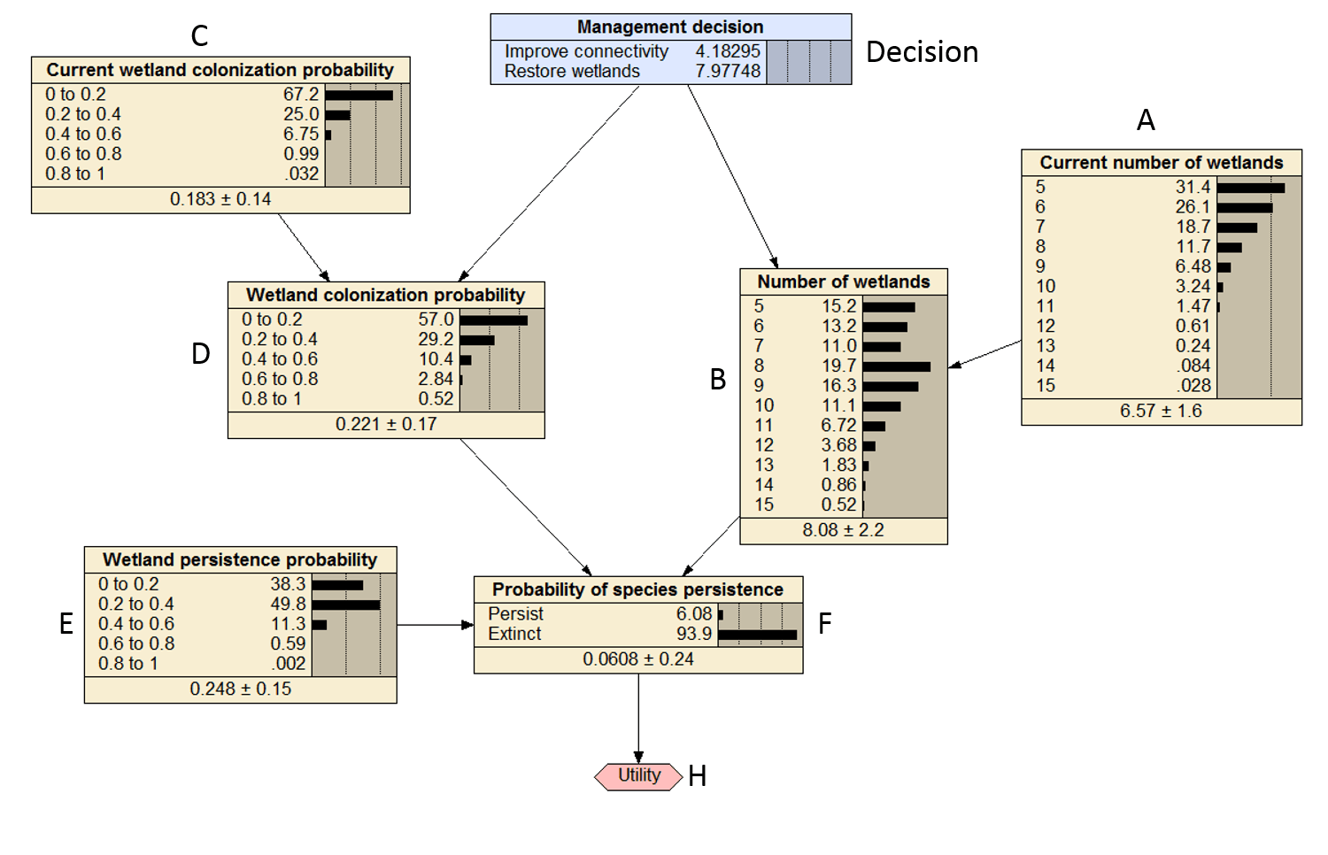
Figure 1. Compiled Bayesian decision network that was replicated in R.
For each of the lettered nodes in Figure 1 there are conditional probably tables associated with each. The code below reads in the CPT for each node. Note this may be a vector of probabilities for nodes like C or a table of the probabilities of all the possible outcomes for a node like D.
A<-read.xlsx("bdn-tables.xlsx",sheet="current number wetlands")
A[,-c(1)]<-A[,-c(1)]/100
I took the numbers directly from the CPT for A in Netica, copy and paste, which are reported as % so the second line of code converts all the percentages to probabilities varying from 0 to 1. Below is what the A table looks like
A
##    number.of.wetlands  probablity
## 1                   5 0.313650000
## 2                   6 0.261375000
## 3                   7 0.186696000
## 4                   8 0.116685000
## 5                   9 0.064825100
## 6                  10 0.032412500
## 7                  11 0.014733000
## 8                  12 0.006138740
## 9                  13 0.002361050
## 10                 14 0.000843233
## 11                 15 0.000281078
## 12                  5 0.313650000
## 13                  6 0.261375000
## 14                  7 0.186696000
## 15                  8 0.116685000
## 16                  9 0.064825100
## 17                 10 0.032412500
## 18                 11 0.014733000
## 19                 12 0.006138740
## 20                 13 0.002361050
## 21                 14 0.000843233
## 22                 15 0.000281078
Now I repeat the process for all the lettered nodes in Figure 1. I do not have to anything for the decision or utility node. In this case the utility is simply the probability of persistence x 100 which is easy enough to calculate in R. If there were elicited values then that table would need to be imported as well. The code below imports the remaining nodes and coverts them to probabilities.
B<-read.xlsx("bdn-tables.xlsx",sheet="number of wetlands")
B[,-c(1:2)]<-B[,-c(1:2)]/100
C<-read.xlsx("bdn-tables.xlsx",sheet="Current wetland colonization pr")
C[,-1]<-C[,-1]/100
D<-read.xlsx("bdn-tables.xlsx",sheet="Wetland colonization probabilit")
D[,-c(1:2)]<-D[,-c(1:2)]/100
E<-read.xlsx("bdn-tables.xlsx",sheet="Wetland persistence probability")
E[,-1]<-E[,-1]/100
F<-read.xlsx("bdn-tables.xlsx",sheet="prob. spp. persistence")
Here is how a more complicated node that is the child of 2 parents looks.
B
##                decision current.number.wetlands           5           6
## 1  Improve connectivity                       5 8.80537e-01 1.19167e-01
## 2  Improve connectivity                       6 1.06479e-01 7.86778e-01
## 3  Improve connectivity                       7 2.63865e-04 1.06451e-01
## 4  Improve connectivity                       8 1.19795e-08 2.63865e-04
## 5  Improve connectivity                       9 9.96126e-15 1.19795e-08
## 6  Improve connectivity                      10 1.51710e-22 9.96126e-15
## 7  Improve connectivity                      11 4.23190e-32 1.51710e-22
## 8  Improve connectivity                      12 1.17549e-38 4.23190e-32
## 9  Improve connectivity                      13 0.00000e+00 1.17549e-38
## 10 Improve connectivity                      14 0.00000e+00 0.00000e+00
## 11 Improve connectivity                      15 0.00000e+00 0.00000e+00
## 12     Restore wetlands                       5 1.19795e-08 2.63865e-04
## 13     Restore wetlands                       6 9.96126e-15 1.19795e-08
## 14     Restore wetlands                       7 1.51710e-22 9.96126e-15
## 15     Restore wetlands                       8 4.23190e-32 1.51710e-22
## 16     Restore wetlands                       9 1.17549e-38 4.23190e-32
## 17     Restore wetlands                      10 0.00000e+00 1.17549e-38
## 18     Restore wetlands                      11 0.00000e+00 0.00000e+00
## 19     Restore wetlands                      12 0.00000e+00 0.00000e+00
## 20     Restore wetlands                      13 0.00000e+00 0.00000e+00
## 21     Restore wetlands                      14 0.00000e+00 0.00000e+00
## 22     Restore wetlands                      15 0.00000e+00 0.00000e+00
##              7           8           9          10          11          12
## 1  2.95386e-04 1.34105e-08 1.11512e-14 1.69833e-22 4.73744e-32 1.17549e-38
## 2  1.06479e-01 2.63935e-04 1.19826e-08 9.96389e-15 1.51750e-22 4.23301e-32
## 3  7.86571e-01 1.06451e-01 2.63865e-04 1.19795e-08 9.96126e-15 1.51710e-22
## 4  1.06451e-01 7.86571e-01 1.06451e-01 2.63865e-04 1.19795e-08 9.96126e-15
## 5  2.63865e-04 1.06451e-01 7.86571e-01 1.06451e-01 2.63865e-04 1.19795e-08
## 6  1.19795e-08 2.63865e-04 1.06451e-01 7.86571e-01 1.06451e-01 2.63865e-04
## 7  9.96126e-15 1.19795e-08 2.63865e-04 1.06451e-01 7.86571e-01 1.06451e-01
## 8  1.51710e-22 9.96126e-15 1.19795e-08 2.63865e-04 1.06451e-01 7.86571e-01
## 9  4.23190e-32 1.51710e-22 9.96126e-15 1.19795e-08 2.63865e-04 1.06451e-01
## 10 1.17549e-38 4.23301e-32 1.51750e-22 9.96389e-15 1.19826e-08 2.63935e-04
## 11 0.00000e+00 1.17549e-38 4.73745e-32 1.69834e-22 1.11513e-14 1.34106e-08
## 12 1.06451e-01 7.86571e-01 1.06451e-01 2.63865e-04 1.19795e-08 9.96126e-15
## 13 2.63865e-04 1.06451e-01 7.86571e-01 1.06451e-01 2.63865e-04 1.19795e-08
## 14 1.19795e-08 2.63865e-04 1.06451e-01 7.86571e-01 1.06451e-01 2.63865e-04
## 15 9.96126e-15 1.19795e-08 2.63865e-04 1.06451e-01 7.86571e-01 1.06451e-01
## 16 1.51710e-22 9.96126e-15 1.19795e-08 2.63865e-04 1.06451e-01 7.86571e-01
## 17 4.23190e-32 1.51710e-22 9.96126e-15 1.19795e-08 2.63865e-04 1.06451e-01
## 18 1.17549e-38 4.23301e-32 1.51750e-22 9.96389e-15 1.19826e-08 2.63935e-04
## 19 0.00000e+00 1.17549e-38 4.73745e-32 1.69834e-22 1.11513e-14 1.34106e-08
## 20 0.00000e+00 1.17549e-38 4.73745e-32 1.69834e-22 1.11513e-14 1.34106e-08
## 21 0.00000e+00 1.17549e-38 4.73745e-32 1.69834e-22 1.11513e-14 1.34106e-08
## 22 0.00000e+00 1.17549e-38 4.73745e-32 1.69834e-22 1.11513e-14 1.34106e-08
##             13          14          15
## 1  0.00000e+00 0.00000e+00 0.00000e+00
## 2  1.17549e-38 0.00000e+00 0.00000e+00
## 3  4.23190e-32 1.17549e-38 0.00000e+00
## 4  1.51710e-22 4.23190e-32 1.17549e-38
## 5  9.96126e-15 1.51710e-22 4.23190e-32
## 6  1.19795e-08 9.96126e-15 1.51710e-22
## 7  2.63865e-04 1.19795e-08 9.96126e-15
## 8  1.06451e-01 2.63865e-04 1.19795e-08
## 9  7.86571e-01 1.06451e-01 2.63865e-04
## 10 1.06479e-01 7.86778e-01 1.06479e-01
## 11 2.95387e-04 1.19168e-01 8.80537e-01
## 12 1.51710e-22 4.23190e-32 1.17549e-38
## 13 9.96126e-15 1.51710e-22 4.23190e-32
## 14 1.19795e-08 9.96126e-15 1.51710e-22
## 15 2.63865e-04 1.19795e-08 9.96126e-15
## 16 1.06451e-01 2.63865e-04 1.19795e-08
## 17 7.86571e-01 1.06451e-01 2.63865e-04
## 18 1.06479e-01 7.86778e-01 1.06479e-01
## 19 2.95387e-04 1.19168e-01 8.80537e-01
## 20 2.95387e-04 1.19168e-01 8.80537e-01
## 21 2.95387e-04 1.19168e-01 8.80537e-01
## 22 2.95387e-04 1.19168e-01 8.80537e-01
Solving the BDN
To solve the BDN I need to work iteratively from parent to child node and calculate the marginal probabilities for each parent node to combine with the CPT of the child node. The marginal probabilities are the belief bars that are illustrated for each node in Figure 1.
Marginal probability of wetland colonization probability (B)
The marginal probability for node B (Number of wetlands) is calculated by combining the probability for current number of wetlands (A) and conditional on the management decision. Now the management decision does not effect the current number of wetlands but it does influence the future number of wetlands (B) as you can see in the CPT for B above. The trick to doing the calculations efficiently is to use matrix multiplication. Some quick notes on the matrix multiplication.
- the dimensions of B is 22 rows by 11 columns
- the dimensions of A is technically 11 rows by 1 column for the 11 states in node A, but above it has 22 rows!
- the number of decisions is 2
For the matrix multiplication to work A must be 22 rows by 1 to match the number of rows in B. Why 22? Well this is because of the decision node is connected to node B and therefore we need to repeat the probabilities for A to account for each decision! Now it is efficient to use matrix multiplication to multiply the marginal probabilities of A and the conditional probabilities of B as below. Note I am doing the matrix multiplication only on the probabilities.
# marginal probabilities for B
B_mp<-t(B[,-c(1,2)])%*%A[,-1] ## probability of each outcome given the inputs
# divide by the sum to
B_mp<-B_mp/sum(B_mp) # the denominator is the marginal likelihood, serves to normalize and sum to 1
# for easy handling later.
B_mp<-data.frame(state=names(B[,-c(1,2)]),prob=B_mp)
The marginal probabilities for B are the same as the ones specified in figure 1. Cool beans.
B_mp
##    state        prob
## 5      5 0.152030152
## 6      6 0.131504031
## 7      7 0.110334337
## 8      8 0.196606849
## 9      9 0.162898512
## 10    10 0.110595162
## 11    11 0.067171590
## 12    12 0.036785601
## 13    13 0.018301072
## 14    14 0.008577902
## 15    15 0.005194791
Solving the rest of the nodes
Now to solve the rest of the model you simply keep working iterative from parent to child node until you get to the end! The code below does for node D that.
# marginal probabilities for D
D_mp<- t(D[,-c(1,2)])%*%C[,-1]
D_mp<-D_mp/sum(D_mp)
D_mp<-data.frame(state=names(D[,-c(1,2)]),prob=D_mp)
D_mp
##           state        prob
## 0-0.2     0-0.2 0.570384868
## 0.2-0.4 0.2-0.4 0.292496288
## 0.4-0.6 0.4-0.6 0.103609503
## 0.6-0.8 0.6-0.8 0.028355151
## 0.8-1     0.8-1 0.005154191
Node F is a bit more complicated because there are 3 parent nodes (E, D, B). But we first identify all the possible combinations of E, D, and B. Then we assign the marginal probability for E and D calculated above and since B is a just a vector or probabilities we use it.
# marginal probabilities for F
parents<-list(D_mp,B_mp,E)
tmp <- lapply(parents,function(x){1:nrow(x)})
tmp<- expand.grid(tmp)
Now we need to make sure the order of our combinations match the CPT we extracted for F from Netica.
tmp<- tmp[order(tmp[,1],tmp[,2],tmp[,3]),]
Now that is taken care of we assign the correct probability to
each state in tmp.
parents_probs<- tmp
parents_probs[,1]<- parents[[1]][tmp[,1],]$prob
parents_probs[,2]<- parents[[2]][tmp[,2],]$prob
parents_probs[,3]<- parents[[3]][tmp[,3],]$prob
The product of the rows of parents_probs should
sum to 1. Let’s confirm.
sum(apply(parents_probs,1,prod))
## [1] 0.9999995
Now that we have the probability for each possible outcome of node B, D, and E we can use matrix multiplication to calculate the marginal probability for node F of Figure 1.
F_mp<- t(F[,-c(1:3)])%*%apply(parents_probs,1,prod)
F_mp<-F_mp/sum(F_mp)
F_mp
##               [,1]
## persist 0.07165562
## extinct 0.92834438
The utility value is now F_mp times 100. Note that this will be a different calculation if the utility is not a calculated value (i.e., elicited values).
U<-F_mp*100
U
##              [,1]
## persist  7.165562
## extinct 92.834438
But the values of U do not match the numbers in the decision box! What is going on there? Well we need to solve the network for each decision to get the decision specific utility. The utility above is essential the expected utility if you did not know what decision to do.
Solving the network for each decision
Decision: improve connectivity
To solve the network for each decision we just need to ‘turn off’ each decision and solve the matrix. This is easily done by zeroing out the probabilities associated with the decision. Based on Figure 1 the the decision influences node D and B and therefore we need to add a vector to those calculations to represent the decision. The code chunks below solve the BDN if the decision was to ‘improve connectivity’ and ‘restore wetlands’ respectively.
First thing we are going to do is make a vector to hold our utilities.
# utility values: H
U<- rep(0,2) # utility for each decision
Now we can solve the BDN for the first decision.
## decision == improve connectivity
decision<-"Improve connectivity"
# marginal probabilities for B
dec<-ifelse(B[,1]==decision,1,0)
B_mp<-t(B[,-c(1,2)]*dec)%*%A[,-1]
B_mp<-B_mp/sum(B_mp)
B_mp<-data.frame(state=names(B[,-c(1,2)]),prob=B_mp)
### marginal probabilities for D
dec<-ifelse(D[,1]==decision,1,0)
D_mp<- t(D[,-c(1,2)]*dec)%*%C[,-1]
D_mp<-D_mp/sum(D_mp)
D_mp<-data.frame(state=names(D[,-c(1,2)]),prob=D_mp)
### marginal probabilities for F
parents<-list(D_mp,B_mp,E)
tmp <- lapply(parents,function(x){1:nrow(x)})
tmp<- expand.grid(tmp)
tmp<- tmp[order(tmp[,1],tmp[,2],tmp[,3]),]
parents_probs<- tmp
parents_probs[,1]<- parents[[1]][tmp[,1],]$prob
parents_probs[,2]<- parents[[2]][tmp[,2],]$prob
parents_probs[,3]<- parents[[3]][tmp[,3],]$prob
F_mp<- t(F[,-c(1:3)])%*%apply(parents_probs,1,prod)
F_mp<-F_mp/sum(F_mp)
And now we grab the utility
U[1]<- F_mp[1]*100
The marginal probabilities calculate above should all be close to the marginal probabilities in Figure 2 below.
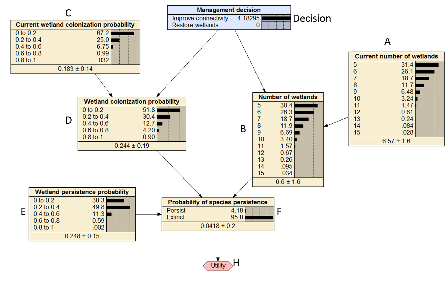
Figure 2. Compiled Bayesian decision network that was replicated in R with the decision set to improve connectivity.
Decision: restore wetlands
Now on to the next decision
## decision == restore wetlands
decision<-"Restore wetlands"
# marginal probabilities for B
dec<-ifelse(B[,1]==decision,1,0)
B_mp<-t(B[,-c(1,2)]*dec)%*%A[,-1]
B_mp<-B_mp/sum(B_mp)
B_mp<-data.frame(state=names(B[,-c(1,2)]),prob=B_mp)
### marginal probabilities for D
dec<-ifelse(D[,1]==decision,1,0)
D_mp<- t(D[,-c(1,2)]*dec)%*%C[,-1]
D_mp<-D_mp/sum(D_mp)
D_mp<-data.frame(state=names(D[,-c(1,2)]),prob=D_mp)
### marginal probabilities for F
parents<-list(D_mp,B_mp,E)
tmp <- lapply(parents,function(x){1:nrow(x)})
tmp<- expand.grid(tmp)
tmp<- tmp[order(tmp[,1],tmp[,2],tmp[,3]),]
parents_probs<- tmp
parents_probs[,1]<- parents[[1]][tmp[,1],]$prob
parents_probs[,2]<- parents[[2]][tmp[,2],]$prob
parents_probs[,3]<- parents[[3]][tmp[,3],]$prob
F_mp<- t(F[,-c(1:3)])%*%apply(parents_probs,1,prod)
F_mp<-F_mp/sum(F_mp)
And we now get that utility.
U[2]<- F_mp[1]*100
The values are darn close to the values in Figure 1 of 4.1 and 8.0.
U
## [1] 4.309007 9.287041
There is some discrepancy on the last utility 9.2 versus 8.0, which i think is due to some rounding errors in the CPT of D. The marginal probabilities calculate above should all be close to the marginal probabilities in Figure 2 below.

Figure 3. Compiled Bayesian decision network that was replicated in R with the decision set to restore wetlands.
References
Conroy, M. J., and J. T. Peterson. 2013. Decision making in natural resource management: a structured, adaptive approach. Wiley.